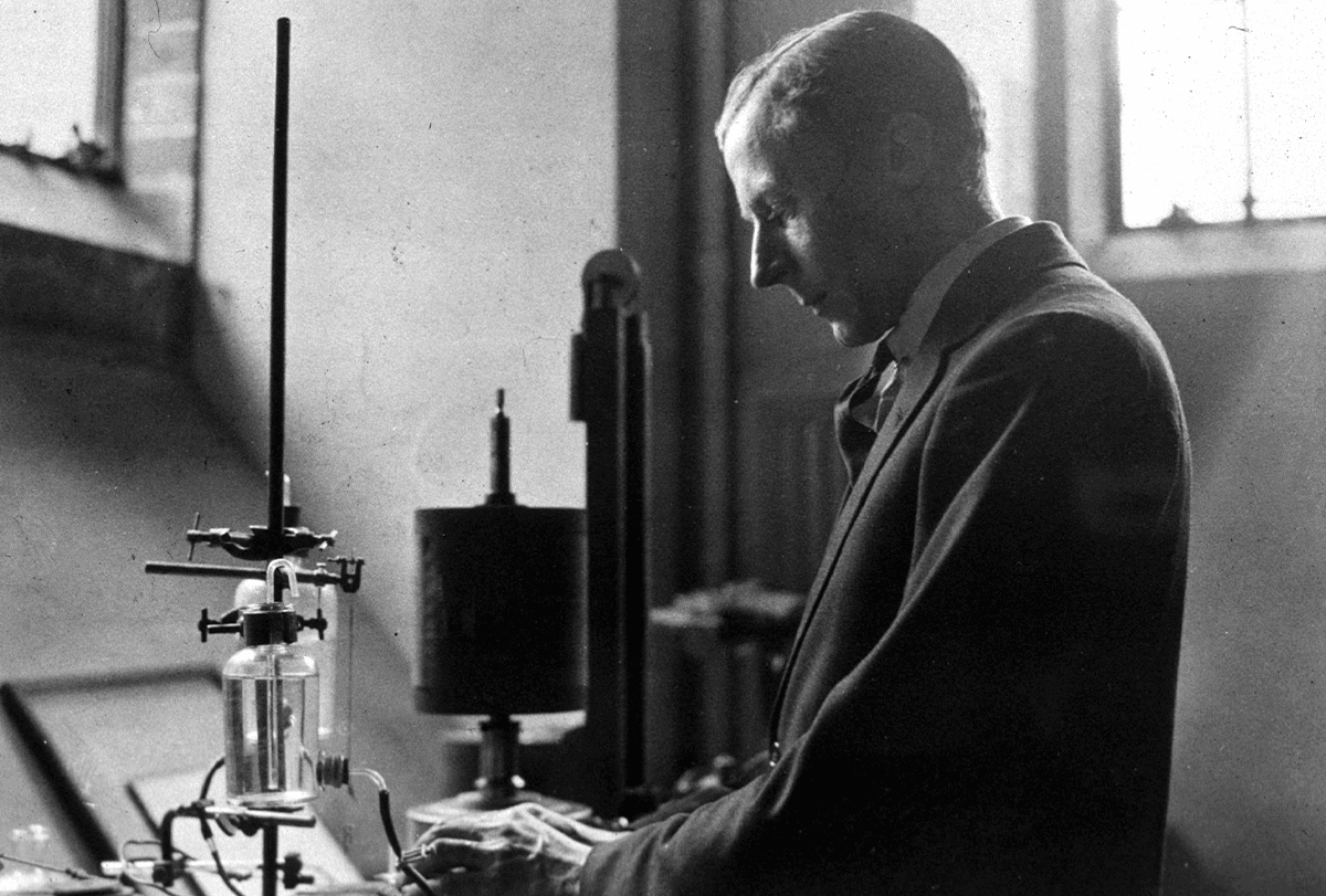
Edgar Adrian works in the laboratory, around 1920.
In focus: Edgar Douglas Adrian works in the laboratory, around 1920.
Science History Images / Alamy Stock Photo
Add us as a Preferred Source on Google

The neural code at 100

In two 1926 articles, Edgar Douglas Adrian revealed that neurons communicate through trains of spikes.

By Matteo Carandini
12 October 2026 | 8 min read

“We were excited, both of us quite aware that what we now saw had never been observed before and that we were discovering a great secret of life.” Such was the atmosphere in 1925 in a basement in Cambridge, England, where Yngve Zotterman, a 27-year-old trainee with a gift for dissection, had just helped Edgar Douglas Adrian perform the experiment of the century. They had discovered the neural code. 

Zotterman had moved to England only two months earlier, drawn by Adrian’s studies on the “all-or-none” response of nerves. In these studies, Adrian and his own mentor, Keith Lucas, had observed that the current applied to a motor nerve contracted the attached muscle only if it exceeded a minimum value, above which the effect would be no stronger. This all-or-none property was somehow due to the nerve itself and seemed to apply to all nerves, not just the motor ones.

We now understand this all-or-none event as the action potential, or spike. But in the early 1920s, spikes had been observed only by applying strong currents to whole nerves, which made many axons fire at the same time. Only then was the resulting aggregate spike large enough for the instruments to detect. Scientists did not yet know that individual axons carry spikes during their normal function, that these spikes have a fixed shape, that they form sequences, and that these sequences form a code. 

The key problem was amplification: Spikes are tens of millivolts in size intracellularly but about a thousand times smaller extracellularly. Fortunately, a hot new technology developed for radio in the 1920s—the vacuum valve—offered a solution. Neurophysiologists at Harvard University and Washington University had started using these valves to amplify nerve signals, with promising results. 

When Adrian first applied the valve-based amplifier in his recordings, however, he became dejected; the electrical fluctuations he saw in a motor nerve seemed random and artifactual. But he soon noticed that these fluctuations appeared only when the muscle serving the motor nerve was stretched. As he later recalled: “The explanation suddenly dawned on me [that I was recording] sensory impulses [sent] up the nerves coming from the muscle spindles, signalling the stretch on the muscle.” Adrian had just recorded the first spike trains: sequences of spikes produced by neurons and transmitted through their axons. But his recordings contained the activity of many neurons simultaneously; the activity of single fibers—the axons of single neurons—remained a mystery. He was “nearly certain that many of these [fluctuations]  were action potentials coming up sensory fibres in the nerve, and what was more, that many of them came from single nerve fibres and that by some extension of the technique it ought to be possible to find out exactly what was happening in single nerve fibres.”

These hopes were fulfilled, thanks to Zotterman’s gift for dissection. During a recording from a motor nerve, Zotterman progressively cut away more sections of the attached muscle until the remaining section contained a single spindle. The fluctuations observed in the nerve suddenly changed: They were all the same shape; they were quite regular; and their frequency grew when the muscle was stretched. 

With this recording, Adrian and Zotterman had discovered the language of neurons: the digital code of ones and zeros that we call the neural code. They had discovered that an individual neuron signals the quantity of interest through spikes, and that when that quantity changes, the neuron changes the frequency—not the size—of those spikes. These striking results were published in two papers in 1926 that were immediately recognized as transformational, earning Adrian a Nobel Prize a mere six years later. 

I

t was a massive discovery, and yet the images that proved it are cryptic to our modern eye. When Adrian and Zotterman recorded the spikes carried by multiple axons, they saw the traces shown here, in panel A. When the muscle was progressively reduced to contain a single spindle so that only one of the axons carried spikes, they obtained the traces in panel D. They saw this as a eureka moment, revealing that “great secret of life,” and yet we would find it hard to share that enthusiasm: The figures are hard for us to parse.
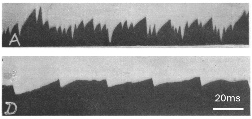
The first spontaneous spikes, recorded using a capillary electrometer.
Trace discovery: Scientists used a “capillary electrometer,” which has a low temporal resolution, to record the first spontaneous spikes, creating graphs unfamiliar to modern neuroscientists. The top image shows spikes from multiple axons. The bottom image shows spikes from a single axon. In this image, time runs from right to left.
Modified from Adrian and Zotterman, 1926

The culprit is the slow reporting device used in the recordings, the “capillary electrometer.” This device exploits the tiny movements elicited by voltage in a fine pipette filled with mercury, which are magnified with a microscope, projected and filmed. Adrian chose it because it was robust: It would withstand the amplifier’s occasional wild artifacts. But the mercury level takes time to revert after a fluctuation, effectively blurring the signal in time. Recovering the original signals required deconvolution (similar to modern-day calcium indicators. This deconvolution was performed with a mechanical device but was more often left to the imagination of the experimenters and of their readers. It also does not help that in those figures time runs the wrong way (right to left!).

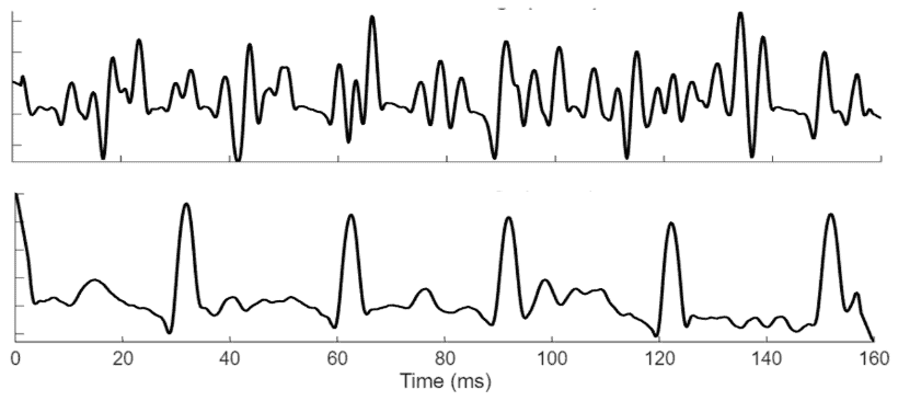
To reveal the glory of these images, I flipped the time axis and deconvolved the traces. In the resulting traces, the spikes become recognizable, although they are still a bit blurred (spikes last a few milliseconds, not tens of milliseconds). And the difference between spikes from multiple axons (top) versus a single axon (bottom) becomes stark. With this more modern visualization, we can now imagine their excitement!

Spikes carried by multiple axons and a single axon.
Modern means: Deconvolving the original traces makes them more recognizable to today’s neuroscientists. Top: Spikes carried by multiple axons. Bottom: Spikes carried by a single axon.
Matteo Carandini

These 1926 discoveries not only revealed the neural code but also shifted the focus from the medium (the nerve) to the message (the neural code). Adrian marveled at its simplicity: “The message consists merely of a series of brief impulses or waves […]. In any one fibre the waves are all of the same form and the message can only be varied by changes in the frequency and duration of the discharge.” He described this code as “scarcely more complex than a succession of dots in the Morse Code.” Or, more vividly: “The nervous message may be likened to a stream of bullets from a machine gun, it cannot be likened to a continuous stream of water from a hose.” 

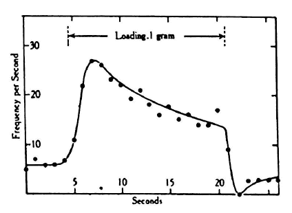
This breakthrough paved the way for fundamental discoveries about the quantities encoded by the firing of neurons, and the first of these appeared in the very same 1926 paper: the progressive decrease in firing observed during steady stimulation, which Adrian termed “adaptation.” To document it, he produced a graph that is readily understandable to us, showing the nerve’s firing rate as a function of time (before, during and after a muscle is stretched).

The first plot of firing rate versus another quantity.
Landmark plot: This graph, published 100 years ago, is the first plot of firing rate versus another quantity. Here that quantity is time, and the plot reveals the phenomenon of adaptation: While the stimulus is constant, the firing rate slows over time.
Adrian and Zotterman, 1926

This graph marks a watershed: It is the first graph of neuronal firing rate plotted against something else. Today, we produce such plots all the time in our laboratories, and we even give them acronyms (this one is a “PSTH”). They are the plots that documented 100 years of foundational discoveries, such as center-surround receptive fields in the retina, orientation selectivity in visual cortex, place fields in the hippocampus, reward-expectation dopamine signals, and grid cells in the entorhinal cortex (can you spot which one has yet to receive the Nobel prize?). And yet, before 1926 these plots would have been impossible, because the quantity on the y axis was not even known to exist!

Happy 100-year anniversary to the neural code. We neuroscientists ought to celebrate it like our biologist friends do for the genetic code (which, incredibly, was discovered 300 meters away!). And yet we take it for granted, as if it was always known. 

Thinking back 100 years to 1926, it is amazing how little scientists knew about the brain at the time. Surely the same will apply 100 years from now, when our successors will be amazed at how little we understood in 2026. Hopefully, they will have discovered another form of neural code: some simple organizational principle that is so pervasive across the brain that it will be hard to fathom a time when it was not known.

Sign up for our weekly newsletter.

Catch up on what you missed from our recent coverage, and get breaking news alerts.